Implicits and fields for beginners
Written by nTop
Published on May 13, 2019
Managing the size and performance of complex geometry requires a computationally lighter means of defining and representing geometry. By integrating a field-driven design approach based on the implicit modeling technology, designers can focus on engineering work that matters, and spend less time with non-value-added tasks.
In CAD environments, geometry can be defined and represented in more ways than one. If you have ever used a 3D modeling program, you've most likely worked with meshes, b-reps, or both depending on the task at hand. Although meshes and b-reps have their strong points, their weaknesses rear their head as geometry becomes more complex. Managing the size and performance of complex geometry requires a computationally lighter means of defining and representing geometry. By integrating a field-driven design approach based on the implicit modeling technology, designers can focus on engineering work that matters, and spend less time with non-value-added tasks.
Implicit geometry
Implicit modeling is a powerful way to define, change, and represent 3D geometry. Geometry is defined through equations, rather than through a network of vertices, edges, and faces like meshes and b-reps. This means that implicits are significantly lighter to compute and maintain their pure form because they are not discretized like meshes and b-reps, which don't always capture continuity perfectly. For instance, mesh geometry, regardless of its resolution is a faceted representation of the actual form. At some point in the design to manufacturing pipeline, some form of discretization will be required, whether it is through meshes, b-reps, or producing slice data for manufacturing. By discretizing data from implicit models directly to a manufacturing-ready output, the discretization occurs at the very end of the process rather than at the beginning or throughout. This means that outgoing manufacturing data is more precise. In addition to being orders of magnitude faster to compute, implicit geometry also results in super lightweight files as only a minimal amount of information is needed.
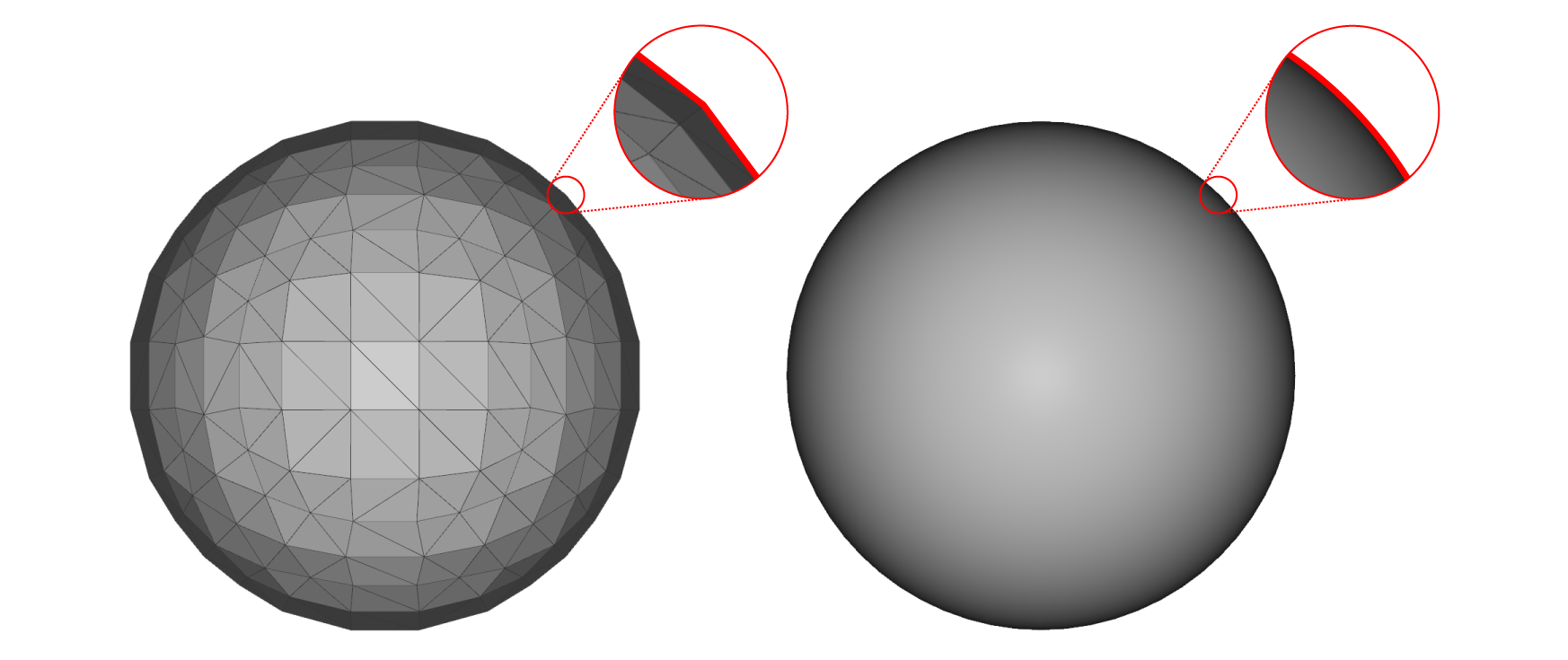
A mesh representation compared to an implicit representation of a sphere. In this example, the mesh face count of the sphere is purposely low to exaggerate the discretization. Even if the mesh face count was significantly increased to more accurately represent the sphere, the file size would also increase.
On-demand geometry rendering in nTop.
Rather than descritizing implicit geometry, sampling and previewing geometry through shaders is a form of rendering that enables users to quickly view geometry at very low or very high resolution. This form of rendering leverages a computer’s graphic processing unit.
Understanding fields
Field-Driven Design is an empowering concept that builds upon implicit modeling. It has several benefits to end users and organizations, such as increased flexibility and efficiency of design. To better understand the concept of fields, let’s first explain how it works by using weather as an analogy. Imagine driving along the east coast of the United States from Florida to Maine, with the goal of finding optimal places to camp along the way based on simple weather data. At each mile, using a weather app, you could sample information such as temperature, wind, humidity, visibility and air quality. Each information type, such as temperature, is continuous, meaning it is everywhere. This is a field, and you can sample this temperature field and all other weather fields at every mile, half-mile, yard, foot, inch, etc. The key takeaway is that we can use one type of weather data or combine all of it to inform our decision on where to camp. In a similar way, fields representing different types of data such as distance, force, or velocity values can be used and even combined to enhance implicit geometry for optimal performance.
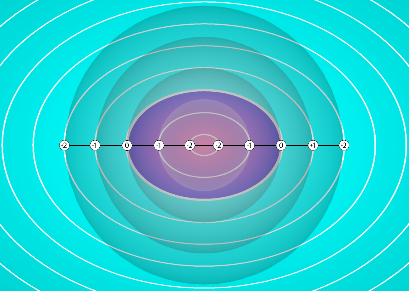
Although many different types of data can be converted into fields, we’ll only focus on distance fields, since they are the first type of field you'll encounter in nTop. When creating models through a visual programming interface, the output is more than just the representation of implicit geometry. Under the hood of each implicit operation resides an equation that outputs the distance values to the boundary of the geometry. Like temperature in our environment, distance data is everywhere. It can be sampled at very large or very small increments from any height or depth in any axis. It is everywhere. Why are these distance values relevant to the representation of geometry? Distance values that equal zero define the boundary of geometry. Negative distance values define what is inside, while positive values define what is outside.
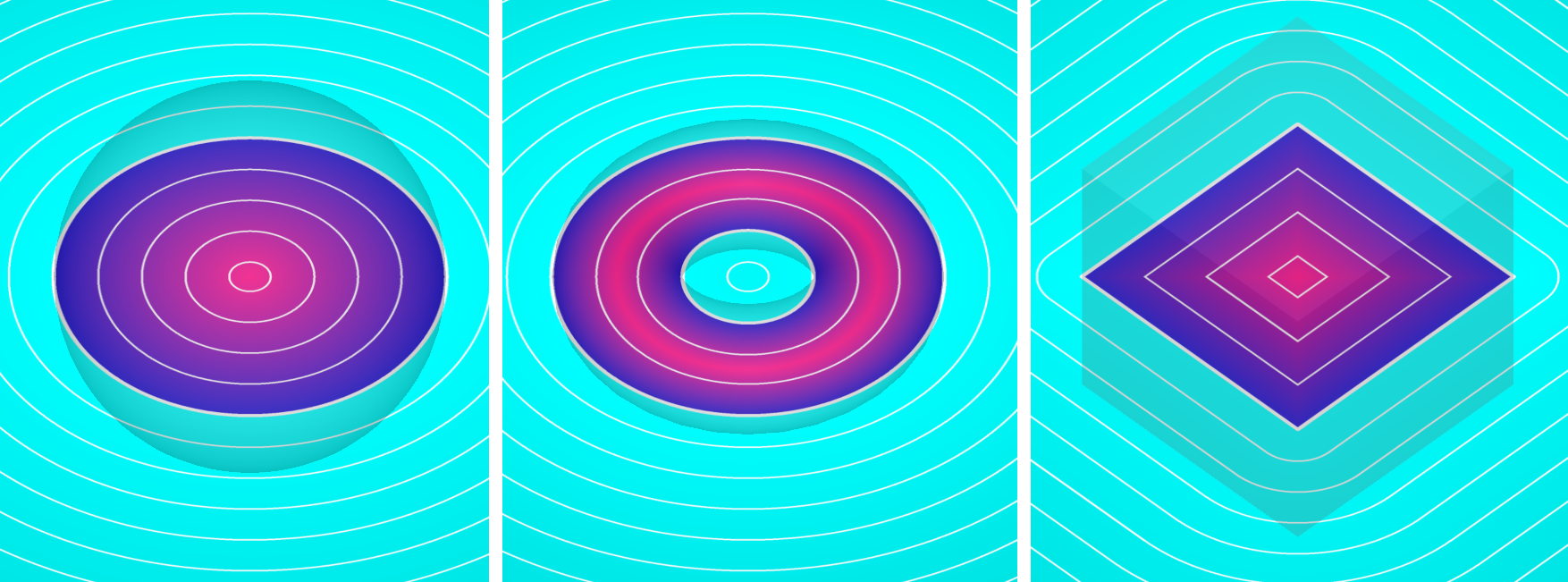
An example of distance fields in nTop, sampled at the cross-section of a sphere, torus, and cube. Values beyond the boundary of each primitive are positive, while values internal are negative. The radiating white lines represent the resolution at which the distance field is sampled, in this case, every 2 millimeters.
Distance fields for modeling operations
Other than the zero values that define the boundary of our geometry, how can the positive and negative values of a field be utilized? Imagine wanting to offset a sphere. We now know that the boundary of the sphere is composed of zeros. If we wanted to offset the sphere by one millimeter, we would need the zero values to be one millimeter away from where they are currently.
In nTop, a user can do this by subtracting one millimeter from a sphere or by using the Offset Implicit block. With field-driven design, there are more avenues for engaging with implicit geometry than with meshes and b-reps in typical modeling paradigms.
In nTop, users can perform operations on implicits mathematically or through specific functional blocks.
Boolean operations are some of the first commands any designer or engineer learns when introduced to 3D modeling. But as we become more skilled, we notice that these incredible commands become more volatile as geometric complexity increases. When boolean unioning one mesh with another, two networks of vertices, edges, and faces are recalculated into one new network.
When boolean unioning two mesh spheres, a new network of vertices, edges, and faces is formed. This network is composed of network geometry from each original sphere and new geometry in order to connect the two.
Combining two simple mesh geometries is easy, but performing this operation among complex mesh parts such as lattices most certainly results in a failure at some point. However, implicit modeling treats these problems entirely differently and they never fail. Computing the boolean union of two geometries implicitly is just a matter of extracting the minimum values of two overlapping distance fields. Inverting this condition to extract the maximum values between the two fields will result in a boolean intersect, as shown below:
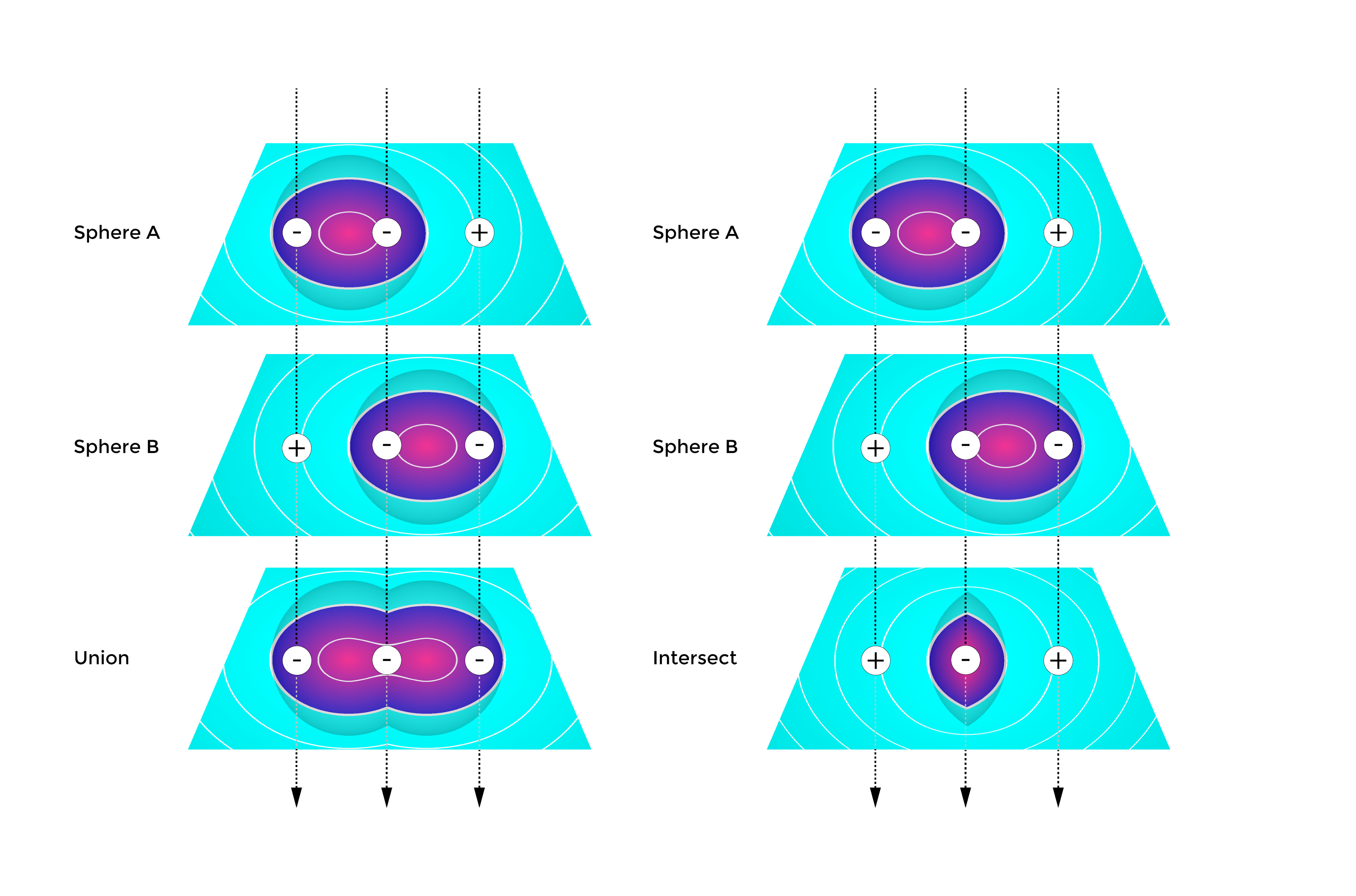
Left: The boolean union of two fields in nTop, which extracts the minimum values between two fields. Right: The boolean intersect of two fields in nTop, which extracts the maximum values between two fields.
Summary
Just as weather data can determine camping conditions, distance fields determine the result of modeling operations, such as booleans, offsets, and fillets to name a few. Engineers and designers using a field-driven approach to driving implicit models are freed from frustrating manual setup, rework and data repair, and have the ability to fine-tune and control their data. They can focus on creative, breakthrough designs with a smooth pathway to manufacturing. From modeling to simulation to manufacturing, fields are ever present in nTop’s core workflows and enable our users to drive geometry with layers of synthesized data.
In future posts we’ll take a closer look at how distance fields, scalar fields, and vector fields work together to generate high performing products. If you’d like to learn about other fields, read our recent blog posts where we showcase how stress fields can drive the strut diameters of a lattice structure in a brake pedal, or how various loading conditions can be combined to vary the diameter of cantilever struts.

nTop
nTop (formerly nTopology) was founded in 2015 with the belief that engineers’ ability to innovate shouldn’t be limited by their design software. Built on proprietary technologies that upend the constraints of traditional CAD software while integrating seamlessly into existing processes, nTop allows designers in every industry to create complex geometries, optimize instantaneously, and automate workflows to develop breakthrough 3D-printed parts in record time.
Related content
- VIDEO
Five ways to lightweight in nTop
- VIDEO
Sneak peek into the nTop + Autodesk Fusion 360 integration
- ARTICLE
Optimizing thermal management with conformal cooling to extend operational life
- ARTICLE
Advancing structural performance of aerospace heat exchangers
- VIDEO
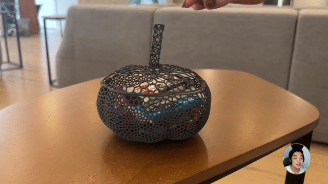
Design a spooky Halloween candy bowl in nTop